Boosting
Boosting methods are a family of ensembling aggregators that take weak (or very dumb) classifiers and make a quite robust one. There are a lot of them, but one of the first ones to appear was AdaBoost.
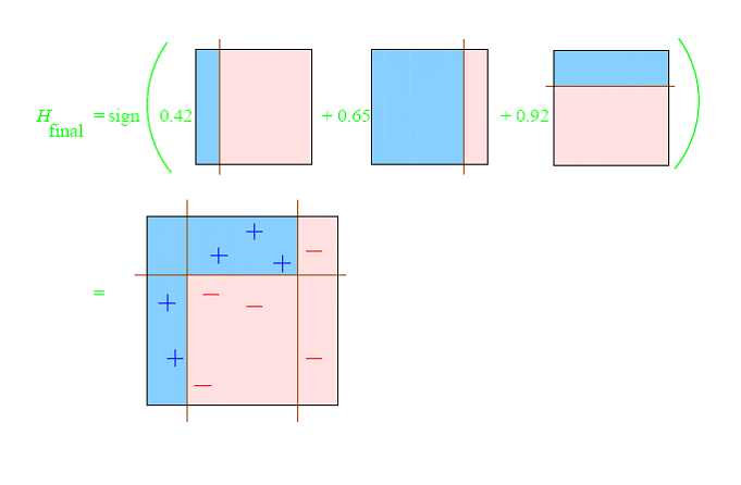
At any given time <math>T</math>, we are aggregating <math>T</math> binary classifiers <math>h_t(\cdot)</math>, and will obtain a new binary classifier with confidence values, that we will then binarize with a sign(·) function.
<math>\widehat{Y} \;\; \epsilon \;\; \mathbb{R}^{NO}</math> taking values <math>\left \{ -1,1\right \}</math>.
The main concept of AdaBoost is to choose <math>T</math> dummy classifiers from a family <math>h_t(\cdot)</math>, and create a weighted average voting. Each classifier will output a numerical value the sign of which will determine the class, and its magnitude will represent the certitude of such classification. The beauty of it is that we can create quite robust classifiers from very dummy, very fast ones.
At any given time <math>T</math>, the linear combination of weak classifiers will look like this:
<math>\widehat{Y}_T = sign(H_T(X)) = sign(\sum_{t<T} \beta_t \cdot h_t(X)) </math>
The trick will be to choose which <math>h_j(\cdot)</math> dummy classifiers to pick (and in which order) and how to come up with the optimal weights <math>\beta_t</math> to combine them.
Note: we will be using subindex <math>m</math> to refer to training examples <math>X_m</math> and their corresponding supervised output <math>Y_m</math>, the subindex <math>j</math> to refer to the given set of <math>h_j(\cdot)</math> weak classifiers, and the subindex <math>t</math> to the order in which we pick each <math>h_t(\cdot)</math> classifier for every given iteration <math>t</math>.
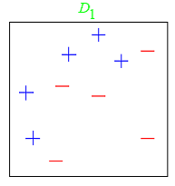
AdaBoost "iteratively adds classifiers, each time reweighting the dataset to focus the next classifier on where the current set makes errors" [UPenn]. The iteration will stop when we start overfitting (cross-validation).
Step 0 - Initialization
Let's define the weights assigned to every training example <math>m</math>:
<math>\omega_m=\frac{1}{M}</math>
And initialize:
<math>t = 0</math>
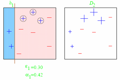
Step 1 - Choosing a new weak classifier
Given the current weighting of the examples <math>\omega_m</math>, we compute the error <math>\epsilon_j</math> of each remaining weak classifier <math>h_j(\cdot)</math> as:
<math>\epsilon_j = \underset{m}{\sum} \omega_m \cdot e^{-Y_m \cdot h_j(Xm)}</math>
For every training example <math>m</math>, the error <math>\epsilon_j</math> will be adding <math>e</math> for those misclassified examples and <math>\frac{1}{e}</math> for the correctly classified, all in a weighted average with <math>\omega_m</math>, that will make previously misclassified examples more important.
From all of the <math>\epsilon_j</math> errors, we will choose the classifier <math>j</math> that leads to less error and will name it <math>h_t(\cdot)</math>.
Step 2 - Adding weak classifier <math>h_t(\cdot)</math> to the ensemble
We have previously defined the ensemble raw output (without the final <math>sign(\cdot)</math> function), as:
<math>H_T(X_m) = \underset{t<T}{\sum }\beta_t \cdot h_t(X_m)</math>
Now we just have to add the next dummy classifier <math>h_t(\cdot)</math> by:
<math>H_t(X_m) = H_{t-1}(X_m) + \beta_t \cdot h_t(X_m)</math>
A good choice of <math>\beta_t</math> being:
<math>\beta_t =\frac{1}{2} \cdot log(\frac{1-\epsilon_t}{\epsilon_t})</math>
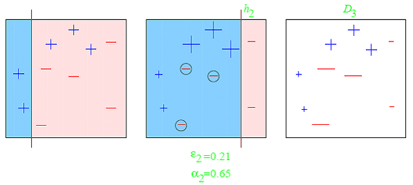
Step 3 - Updating the importance of examples
<math>\omega_{m,t+1}=\omega_{m,t} \cdot e^{Y_m \cdot sign(H_t(X_m))}</math>
<math>t = t+1</math>
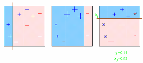
AdaBoost was one of the first successes on proving that very weak (or dummy) classifiers can be aggregated to create a better classifier, that vastly outperforms the dummies.
It is fast to perform thanks to the weakness of the classifiers, their linear aggregation, and the feature selection done by choosing the most performant dummy classifiers.
There is a great number of variants out there. Some of them come up with different heuristics for the weights, some others perform some pruning. There is even a variant using Logistic Regression.
The speed of the algorithm comes at a generalization cost. There is no mathematical framework to analyze the overlap between dummy classifiers, and the classification gain versus computational complexity plateaus at some point.